ML-Density Estimation

Nonparametric Density Estimation

For a random vector x, assuming that it obeys an unknown distribution p(x), the probability of falling into a small area R in the space is

$$P={\int }_{\mathcal{R}}p(x)dx$$

Given $N$ training samples, Number of samples $K$ falling into the region $\mathcal{R}$ follows a binomial distribution

$$P_K=(\genfrac{}{}{0ex}{}{N}{K})P^K(1-P{)}^{N-K}$$

Approximation when $N$ is very large:

When n is very large, we can approximately think that

$$P\approx \frac{K}{N}$$

Assuming $\mathcal{R}$ is small and $p(x)$ is approximately constant within $\mathcal{R}$:

$$P\approx p(x)V$$

Final approximation for $p(x)$:

$$p(x)\approx \frac{K}{NV}$$

To accurately estimate $p(x)$, it is necessary to make $N$ large enough and $V$ as small as possible. However, the number of samples is generally limited, and too small a region will lead to fewer samples falling into the region, so the estimated probability density is not accurate.

Fixed area size, counting the number falling into different areas, which includes histogram method and kernel method.

the area size so that the number of samples falling into each area is zero is called K-nearest neighbor method.

Histograms as density models

For low dimensional data we can use a histogram as a density model.

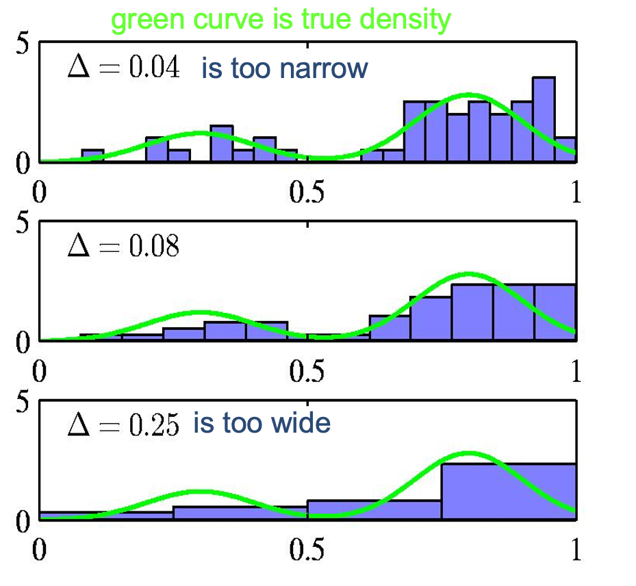
• How wide should the bins be? (width=regulariser)
• Do we want the same bin-width everywhere?
• Do we believe the density is zero for empty bins?

Kernel Density Estimation (KDE)

1. Definition

Kernel Density Estimation (KDE) is a non-parametric method to estimate the probability density function (PDF) of a random variable.

---

2. KDE Formula

$$p(x)=\frac{1}{N}\sum _{n=1}^N\frac{1}{\sqrt{2\pi }H}\exp (-\frac{(x-x_n{)}^2}{2H^2})$$

• $p(x)$: Estimated density at point $x$.
• $N$: Total number of data points.
• $H$: Bandwidth, controlling the smoothness of the density.
• $x_n$: Data points.
• The kernel function $\varphi$ is typically Gaussian:$$\varphi \left(\frac{x-x_n}{H}\right)=\frac{1}{\sqrt{2\pi }H}\exp (-\frac{(x-x_n{)}^2}{2H^2})$$

---

3. Steps to Compute KDE

1. For each data point $x_n$, calculate the distance from the target point $x$.
2. Apply the kernel function to determine the weight of each data point.
3. Sum the contributions from all data points and normalize by $N$.

---

4. Example

Data

We have 5 data points:

$$x=\{1.0,1.5,2.0,3.0,3.5\}$$

We want to estimate the density at $z=2.5$, using:

• Bandwidth $H=0.5$,
• Gaussian kernel.

Calculation

For each $x_n$, calculate:

$$\varphi \left(\frac{z-x_n}{H}\right)=\frac{1}{\sqrt{2\pi }H}\exp (-\frac{(z-x_n{)}^2}{2H^2})$$

• For $x_1=1.0$:

  $$\varphi \left(\frac{2.5-1.0}{0.5}\right)=\frac{1}{\sqrt{2\pi }\cdot 0.5}\exp (-\frac{(2.5-1.0{)}^2}{2\cdot {0.5}^2})\approx 0.008$$

• For $x_2=1.5$:

  $$\varphi \left(\frac{2.5-1.5}{0.5}\right)=\frac{1}{\sqrt{2\pi }\cdot 0.5}\exp (-\frac{(2.5-1.5{)}^2}{2\cdot {0.5}^2})\approx 0.107$$

• For $x_3=2.0$:

  $$\varphi \left(\frac{2.5-2.0}{0.5}\right)=\frac{1}{\sqrt{2\pi }\cdot 0.5}\exp (-\frac{(2.5-2.0{)}^2}{2\cdot {0.5}^2})\approx 0.483$$

• For $x_4=3.0$:

  $$\varphi \left(\frac{2.5-3.0}{0.5}\right)=\frac{1}{\sqrt{2\pi }\cdot 0.5}\exp (-\frac{(2.5-3.0{)}^2}{2\cdot {0.5}^2})\approx 0.483$$

• For $x_5=3.5$:

  $$\varphi \left(\frac{2.5-3.5}{0.5}\right)=\frac{1}{\sqrt{2\pi }\cdot 0.5}\exp (-\frac{(2.5-3.5{)}^2}{2\cdot {0.5}^2})\approx 0.107$$

Combine Contributions

The total density at $z=2.5$ is:

$$p(z)=\frac{1}{N}\sum _{n=1}^N\varphi \left(\frac{z-x_n}{H}\right)$$

Substitute values:

$$p(z)=\frac{1}{5}(0.008+0.107+0.483+0.483+0.107)$$$$p(z)=\frac{1}{5}\cdot 1.188\approx 0.238$$

---

5. Advantages of KDE

• Flexible: Does not assume a specific distribution of data.
• Smooth: Produces a continuous estimate.

6. Challenges of KDE

• Bandwidth $H$: Choosing an appropriate $H$ is critical.
  • Small $H$: May overfit, capturing noise.
  • Large $H$: May oversmooth, losing details.
• Computationally Expensive: Requires evaluating kernel functions for all data points.

---

Summary

In this example, the estimated density at $z=2.5$ is $p(z)\approx 0.238$. Kernel Density Estimation is a powerful tool for non-parametric density estimation, but requires careful parameter tuning.